머신러닝과 딥러닝 BASIC(김성훈 교수님)

1. 기본적인 Machine Learnnig의 용어와 개념 설명

1. Explicit programming(명시적) : 개발자가 일일히 프로그래밍 하는 경우

 

2. Machine learning : 프로그래밍을 하다보면 어떤 경우에는 룰이 너무 많기 때문에 (예_스팸필터, 자율주행) 프로그램 자체가 어떤 데이터를 보고 학습해서 뭔가를 배우는 능력을 갖는 프로그램

 

3. ML의 가장 흔한 문제유형

- 이미지 라벨링 : 태그 된 이미지를 통한 학습

- 이메일 스팸 필터

- 시험성적 예측 : 투자한 시간에 따른 점수 예측

 

4. 학습하는 방법에 따른 Learning 분류

1) Supervised learning 

: Training set (라벨이 정해져 있는 DATA)을 가지고 학습하는 것

예) Cat, dog, mug, hat의 라벨을 붙여 학습

 

- 공부한 시간에 따른 시험성적 예측 : regression

- pass /non-pass 두 개 중에 하나를 고르는 것 : binary classification(분류)

- 공부한 시간에 따른 성적(A,B,C,D,E…) : multi-label classification

 

* Training data set

 

2) Unsupervised learning : un-labeled data

- 구글 뉴스 grouping : 자동적으로 그룹핑을 하기 때문에 일일히 라벨을 정해주기 어렵다

- 워드 클러스트링

 

 

 

2. TensorFlow ( TensorFlow의 설치 및 기본적인 operations)

1. TensorFlow 

: 구글에서 만든 machine intelligence를 위한 오픈소스 라이브러리. 

데이터 플로우 그래프를 사용해서 numerical 계산 가능. 파이썬 언어로 구현 가능

 

2. Data flow graph

- 노드(하나의 오퍼레이션) 간의 연산

- 엣지 : data 배열(=tensor) 간의 연산

 

3. tensorflow 설치

- Linux, max osx, windows : Pip install – upgrade tensorflow

- Source 직접 설치 : Bazel 빌드 프로그램 사용

 

3-1. 설치 및 버전 확인 : 파이썬 실행 후 

Import tensorflow as tf tf.__version__

 

4. TensorFlow mechanics

1) 그래프를 정의한다. placeholder라는 node를 만들 수 있다.

2) sess.run 을 통해 그래프를 실행. (feed_dict={x:x_data})로 값을 넘겨준다

3) 값을 업데이트하거나, 어떤 출력 값을 return한다

- Rank : 0 차원 array s=483

- Shape : 각각 요소에 얼마씩 들어있느냐 / []의 형태로 

예) (3,3) [3,3]

- dtype : 대부분의 경우 float32 / int32

 

3. Linear Regression의 Hypothesis 와 cost

1. Predicting exam score:

Regression model : 

X : 예측하기 위한 기본적인 자료(feature)

Y : 예측을 하는 대상

 

2. Regression → Linear Hypothesis

H(x) = Wx + b (일차방정식) 

→ W와 b에 따라 선의 모양이 달라짐

 

3. H(x) 

: 예측을 어떻게 할 것인가 (hypothesis)

훈련을 많이 할수록 실력이 올라간다

 

4. Linear Regression의 학습이란 : 어떤 선이 이 data를 가장 잘 설명할 수 있는지 그 선을 찾는 것

 

5. Cost function(Loss function) : 어떤 선이 가장 좋은 지

→ 실제 데이터와 가설의 선의 데이터의 잔차 값을 계산

(H(x)-y)^2

 

6. Minimize cost(W,b) : 코스트 값을 최소화하는W,b를 구하는 것이 학습의 목표

 

 

4. Tensorflow로 간단한 linear regression을 구현 (생략)

 

5. Linear Regression의 cost 최소화 알고리즘의 원리

 

1. Hypothesis and cost (어떻게 cost function을 최소화하느냐)

H(x) = Wx + b

 

2. Simplified hypothesis

H(x) = Wx

 

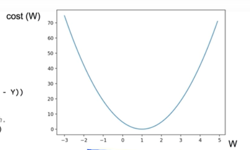
3. cost함수의 모양

W = 1, cost(W)= ? (1 * 1 - )^2 + (1 * 2 – 2)+(1 * 3 – 3) = 0

 

W = 1, cost(W)=0

W = 0, cost(W)=4.67

W = 2, cost(W)=4.67

 

 

- Cost = 0 이 되는 지점을 찾는 것이 목표!

 

4. Gradient descent (경사를 따라 내려가는) 알고리즘

- cost function을 최소화하는데 사용됨

- 경사도를 따라서 아무 값에서나 시작할 수 있다

- W, b를 조금씩 바꿔가며 cost를 줄여가고, 그 과정을 반복한다

- 어떤 점에서 시작하던 간에 항상 최저점에 도달할 수 있는 것이 장점

- 경사도 : 그래프에서 미분한다. 웹사이트(derivative calculator)에서 해준다

- 이 수식을 기계적으로 적용만 시키면 W를 구할 수 있다.

 

5. Convex function (cost function을 3차원으로 표현)

 

 

1) 경사를 타고 내려왔는데 다른 쪽으로 내려올 경우, 알고리즘이 잘 동작하지 않음

2) 이 모양은 어느 점에서 출발해도 항상 최저점을 찾아준다

 

5. Linear Regression의 cost 최소화의 TensorFlow 구현

 

6. multi-variable linear regression

1. Hypothesis using matrix (대문자로 표현)

H(X) = XW

 

2. 실제 data에 적용

 

- [X의 인스턴스 개수, Y의 variable의 개수] * [?, ?] = [5, 1]

- W의 크기를 결정해야 함 → [3, 1]

 

 

3. WX vs XW

- theory

H(x) = Wx + b

 

- TensorFlow(구현)

H(X) = XW

 

 

7. multi-variable linear regression을 TensorFlow에서 구현하기

1. tensorflow code

: 시험 성적 예측

 

 

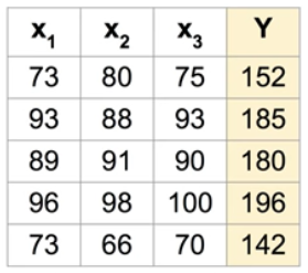
import tensorflow as tf tf.set_random_seed(777)  # for reproducibility x1_data = [73., 93., 89., 96., 73.] x2_data = [80., 88., 91., 98., 66.] x3_data = [75., 93., 90., 100., 70.] y_data = [152., 185., 180., 196., 142.] # placeholders for a tensor that will be always fed. x1 = tf.placeholder(tf.float32) x2 = tf.placeholder(tf.float32) x3 = tf.placeholder(tf.float32) Y = tf.placeholder(tf.float32) w1 = tf.Variable(tf.random_normal([1]), name='weight1') w2 = tf.Variable(tf.random_normal([1]), name='weight2') w3 = tf.Variable(tf.random_normal([1]), name='weight3') b = tf.Variable(tf.random_normal([1]), name='bias') hypothesis = x1 * w1 + x2 * w2 + x3 * w3 + b # cost/loss function cost = tf.reduce_mean(tf.square(hypothesis - Y)) # Minimize. Need a very small learning rate for this data set optimizer = tf.train.GradientDescentOptimizer(learning_rate=1e-5) train = optimizer.minimize(cost) # Launch the graph in a session. sess = tf.Session() # Initializes global variables in the graph. sess.run(tf.global_variables_initializer()) for step in range(2001):     cost_val, hy_val, _ = sess.run([cost, hypothesis, train],                                    feed_dict={x1: x1_data, x2: x2_data, x3: x3_data, Y: y_data})     if step % 10 == 0:         print(step, "Cost: ", cost_val, "\nPrediction:\n", hy_val)

0 Cost:  62547.29 

Prediction:

 [-75.96345  -78.27629  -83.83015  -90.80436  -56.976482]

10 Cost:  14.468626 

Prediction:

 [145.26407 187.59541 178.152   194.48586 145.81136]

…

2000 Cost:  4.897013 

Prediction:

 [148.15846 186.88112 179.63167 195.81955 144.45374] → y data와 유사한 결과값

2. Matrix → H(X) = XW

: 코드는 간결하지만 1과 똑같은 결과

 

import tensorflow as tf tf.set_random_seed(777)  # for reproducibility x_data = [[73., 80., 75.], [93., 88., 93.], [89., 91., 90.], [96., 98., 100.], [73., 66., 70.]] y_data = [[152.], [185.], [180.], [196.], [142.]] # placeholders for a tensor that will be always fed. X = tf.placeholder(tf.float32, shape=[None, 3]) #None=’N개’ Y = tf.placeholder(tf.float32, shape=[None, 1]) W = tf.Variable(tf.random_normal([3, 1]), name='weight') b = tf.Variable(tf.random_normal([1]), name='bias') # Hypothesis hypothesis = tf.matmul(X, W) + b # Simplified cost/loss function cost = tf.reduce_mean(tf.square(hypothesis - Y)) # Minimize optimizer = tf.train.GradientDescentOptimizer(learning_rate=1e-5) train = optimizer.minimize(cost) # Launch the graph in a session. sess = tf.Session() # Initializes global variables in the graph. sess.run(tf.global_variables_initializer()) for step in range(2001):     cost_val, hy_val, _ = sess.run(         [cost, hypothesis, train], feed_dict={X: x_data, Y: y_data})     if step % 10 == 0:         print(step, "Cost: ", cost_val, "\nPrediction:\n", hy_val)

8. TensorFlow로 파일에서 data 읽어오기

 

9. Logistic Classification의 가설 함수 정의

 

* 복습

1. Regression (HCG)

- H (Hypothesis)

- C (Cost 함수)

- G (Gradient decent)

 

2. Classification – 0,1 encoding

1) Spam e-mail Detection : Spam(1) or Ham(0)

 

2) Facebook feed : show(1) or hide(0) 

- ‘좋아요’를 학습하여 좋아할 만한 타임라인만 노출

 

3) Credit Card Fraudulent Transaction detection : legitimate(0), fraud (1) 

- 신용카드를 도난 당했을 때 내가 기존에 많이 사용하던 패턴이냐 아니냐에 따라 가짜를 구별함

 

3. logistic function (sigmoid function)

- H(x) = Wx + b의 결과 값을 0 ~ 1 사이 값으로 만들어주는 함수가 필요

 

→ 다음과 같이 정의

z = WX

H(x) = g(z)

 

4. Logistic Hypothesis (가설)

 

 

 

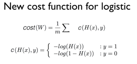
10. Logistic Regression의 cost 함수 설명

 

Global minimum을 찾는 것이 목표